Applying RIP to the Zinc-Finger Mimic

As a first example, we apply RIP to a very small protein, the Zinc-Finger mimic 1FME, an artificial protein that folds into the topology of the zinc finger without the need for zinc.
Setting up the RIP Config File
This is found in the 'examples/zf-mimic' directory. In that directory is a CONFIG file, called 'zf-mimic.config'. It is a config file for a systematic perturbation of the zinc-finger mimic. It is essentially a PYTHON dictionary that will be read by the script PERTURB.PY, and consists of the following:
{ 'raw_pdb':            '1fme.pdb',
  'sim_dir':            '.',
  'force_field':        'AMBER',
  'constraint':         '',
  'n_step_per_pulse':   100,
  'residues':           [],
  'heating_cases':      [('rip', 10, 26, 10000), ('rip', 300, 300, 10000)],
}
The parameters in the file are:
-
'sim_dir' the directory where the results of the simulation will be stored.
-
'raw_pdb' specifies the input PDB that the RIP scripts will pre- process for the AMBER simulation. The script will strip the PDB of hetreo atoms, alternate conformations, hydrogen atoms, and alternative models for NMR files. Then it will process the chain terminii and identify disulfide bonds to produce a PDB file that can be processed by the AMBER program TLEAP, which generates the topology and coordinate start files for the molecular-dynamics proper.
-
'force_field' indicates what MD package is used. In this example, 'AMBER' refers to the AMBER suite, where the bog-standard AMBER force-field is used with the Generalized-Born/Surface-Area implicit solvent force-field is used. The RIP scripts also work with NAMD with explicit solvent but this hasn't really been fleshed out.
-
'n_step_per_pulse' controls how often the RIP perturbation is applied in terms of simulation step-size. As each step is a femtosecond (a standard MD step-size), the pulse for RIP is applied every 100 fs.
-
'constraint' is a command to add positional constraints to the simulation. If set to 'backbone', harmonic constraints will be applied to all backbone atoms. If set to 'surface', harmonic constraints will be applied to all surface and backbone atoms.
-
'residues' indicate the list of residues that will be perturbed. If this list is empty, the RIP scripts will automatically cycle through all amino acids with Χ angles. If you add your own residues, it's very important to remember that the numbering goes from 0, 1, 2, 3... The reason is that counting within PYTHON is always done from 0. Thus 'residues': [0, 23, 54] will apply the perturbation to residue 1, residue 24 and residue 54 of the PDB file. Also this numbering counts sequentially and will ignore gaps.
-
'heating cases' provides the actual parameters for the RIP perturbation. Each case is 4-tuple or a list of four parameters.
-
'rip' chooses the perturbation method. The other choice is 'gas' which is a Langevin thermometer. Use of 'gas' in conjunction with 'surface' constraints will reproduce the original Anisotropic Thermal Diffusion method.
-
The equilibration temperature. Since the method is a highly non-equilibrium process, we only do a rough equilibration. We first apply a langevin thermometer to quickly reach the temperature in 1ps. Then we allow the system to relax at constant energy for 10ps. As RIP is performed in constant energy between each pulse, a constant energy equilibration is needed to allow the structure to escape some kinetic traps only evident in constant energy simulations. Finally, another langevin thermometer is applied for 1ps to bring it to the equilibration temperature.
-
The rotational temperature determines how strongly the rotational velocities are applied. Heuristically, 300K means that the total kinetic energy of the sidechain at 300K is all transferred to the rotational degrees of freedom of the sidechain.
-
The time of the simulation in terms of simulation step-size. 10000 steps (= 10000 fs = 10 ps). The total number of pulses is this value divided by 'n_step_per_pulse'.
-
Running the RIP Simulations
To run, go to the 'pdbtool' directory:
python perturb.py ../examples/zf-mimic/zf-mimic.config
PERTURB.PY will process the RIP protocol encoded in zf-mimic.config, and attempt to run them using AMBER. This simulation took 11 hours on an iMac with a 2.4 GHz Intel processor. After the simulation is done, the .config file will be renamed by adding a '.done' at the end of the filename. The results are stored in
examples/zf-mimic/300k-rip-300k.
In this directory, there will be a series of directories numbered i=1 to 28, each representing the trajectory of a RIP perturbation on residue i in the protein.
I like to group all the files related to a single trajectory with the same basename but different extensions. Thus, all files associated with the trajectory start with 'md'. Analysis scripts can then just refer to 'md' and know where all the associated files are.
Analysis of Flexibility
Of course, you may have your own AMBER trajectory analysis scripts. But if you don't we have several analysis tools provided in the RIP scripts.
The main analysis tool is FLEXIBILITY.PY, if you're in the 'pdbtool' directory, to analyze the 10th (last) picosecond:
python flexibility.py ../examples/zf-mimic/300k-rip-300k 10
It expects the directory structure of the results produced by PERTURB.PY, and will calculate Cα-RMSD of each trajectory, and store these in a file called 'ca_rmsd' for each atom, and in 'ca_rmsd.ave' for each residue. These will be collated in a directory:
examples/zf-mimic/300k-rip-300k/ca_rmsd.10ps
In the analysis, a significant deviation is defined as a Cα-RMSD deviation greater than 6 Å. In this directory, you will find :
-
'map' is an x-y text table of averaged Cα-RMSD values in i'th 'ps where each column represents one of the RIP perturbations. Blank 'columns are inserted for residues that have no perturbable chi 'angles.
-
'limits' gives a calculated background 'min_val' (=mean+2σ), 'as well as the largest deviation 'max_val'.
-
'strength' and 'strength.pdb' measures the number of significant 'responding residues (> 6 Å of Cα-RMSD) for the RIP 'perturbation of each residue. The .pdb file contains the strength 'in the B-factor column
-
'flexibility' and 'flexibility.pdb' measures the susceptibility of a 'residue to large response. It measures number of neighboring RIP 'perturbations that can induce a significant response.
-
'fluctuation' and 'fluctuation.pdb' measures the average amount of 'Cα-RMSD deviation over the simulations where the residue had 'a significant response.
-
a bunch of PDB files named 'x.pdb' that represents the last snapshot of each trajectory where the B-factors represents the averaged Cα-RMSD of that perturbation.
Analysis of Pathways
The main analysis tool for the coupling analysis is PATHWAY.PY, if you're in the 'pdbtool' directory, to analyze the 5th (last) picosecond of the slower simulations:
python flexibility.py ../examples/zf-mimic/10k-rip-26k 5
It expects the directory structure of the results produced by PERTURB.PY, and will calculate the kinetic energy 'kin' of each trajectory, and store these in a file called 'kin.ave' for each residue. These will be collated in a directory:
examples/zf-mimic/10k-rip-26k/kin.5ps
In this directory, you will find:
-
'heatflow_map' is a matrix of numbers. Each i'th column corresponds to a RIP on the i'th residue. The values are the averaged kinetic energy of each residue in the protein of the 5th ps (in this case)
-
'pathway' is a similar matrix to 'heatflow_map' where kinetic energies lower than the background and spurious unconnected residue fluctuations have been supressed to zero
-
'coupling_map' converts 'pathway' into a simple binary matrix where only residues that are hot and connected to the perturbed residues are highlighted with a value of 1, whilst everything else is set to 0
-
'buried_coupling_map', 'tertiary_coupling_map' and 'buried_tertiary_coupling_map' are maps where the couplings in 'coupling_map' have been screened for whether they form tertiary contacts in the folded structure, or are buried relative to the accessible surface area.
-
'*_profile.pdb' are averaged profiles of the corresponding maps over the amino acids. Allows a quick determination of which residues are interesting
Examining the MD trajectories and PDB files
In order to look at trajectories and PDB files, I've developed two convenience scripts that are wrappers around PYMOL.
The first loads trajectories into PYMOL using only a single parameter that refers to the base name of the results of an AMBER trajectory. Furthermore, if a number is given is a second parameter, the script will highlight that residue for better display of the simulation. In this case, we have chosen the perturbation on Phe-12, which produces a very large conformational change:
python pytraj.py ../examples/zf-mimic/300k-rip-300k/12/md 12
This will open a PYMOL window, where the trajectory can be played by clicking on the play button in the bottom right hand corner:
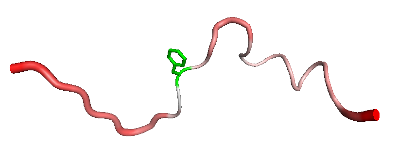
The second script uses PYMOL to display proteins with better default rendering. In the following example, we show the last snapshot of the RIP perturbation to Phe-12, with the residue highlighted in green "-h 12", using a white background "-g white",and displaying the rest of the protein in putty mode where the thickness and color of the backbone indicates the B-factor of the PDB file "-p". Incidentally the B-factor is set to the Cα-RMSD from the initial conformation of the trajectory.k:
 python showpdb.py -p -g white -h 12 ../examples/zf-mimic/300k-
 rip-300k/ca_rmsd.10ps/12.pdb
Both these helper scripts contain various display options that can be viewed by running the scripts with no command-line parameters. Remember to set the location of PYMOL within these scripts as described in the Pre-requisites section.
Generating a Visual Summary
If you've installed all the pre-requisite modules (PYMOL, MATPLOTLIB, MAKO), then you can run the analysis with the '-h' option that tells the program to generate images of the above files, and an HTML file that collates these images
python flexibility.py -h ../examples/zf-mimic/300k-rip-300k 10
This can be viewed through the HTML file examples/zf-mimic/300k-rip-300k/ca_rmsd.10ps/
which should look like this.
Similarly, for the pathway analysis:
python pathway.py -h ../examples/zf-mimic/10k-rip-26k 5
This can be viewed through the HTML file
examples/zf-mimic/10k-rip-26k/kin.5ps/